Contour filters

Many image analysis workflows contain methods that extract shapes that satisfy specific critera. These criteria can be simply based on the corresponding areas of the shapes, through to more complex characteristics such as their associated solidity and eccentricity.

vuba provides a series of contour filters that allow one to extract contour shapes that satisfy some of the aforementioned criteria. These can be serially combined to allow the combination of a variety of criteria and also support pre-defined limits for more fine-scale tuning.

Here, we will cover the basic filters first, followed by the more complex filters that are dependent on additional parameters. For these examples, the following imports are required:

In [1]: import numpy as np

In [2]: import matplotlib.pyplot as plt

In [3]: import cv2

In [4]: import vuba

Basic filters

The basic filters that vuba provides are currently limited to the following: smallest(), largest() and parents().

To demonstrate their usage, we need to first generate some contours to filter:

# Create a handler for the reading from the video
In [5]: video = vuba.Video('../examples/example_data/raw_video/test.avi')

# Read in the first frame and grayscale it
In [6]: first = video.read(index=0, grayscale=True)

# Shrink the roi of the image to remove the time-stamps
In [7]: first = vuba.shrink(first, by=50)

# Threshold the grayscaled frame to a binary threshold (n=50, to=255)
In [8]: _, thresh = cv2.threshold(first, 50, 255, cv2.THRESH_BINARY)

# Find all the contours in the thresholded image
In [9]: contours, hierarchy = vuba.find_contours(thresh, cv2.RETR_TREE, cv2.CHAIN_APPROX_NONE)

The above code has consisted of importing the first frame of the supplied example video and grayscaling it. We then applied a binary threshold to it with a threshold of 50. Note that the threshold applied here is arbitrary and only serves to enable us to generate a variety of shapes. Lastly, we applied contour detection to the thresholded image to generate arrays describing both the coordinates associated with each shape, but also their hierarchial information relative to the other shapes in the image.

Now that we have our contours, we can apply our contour filters and visualise the results!

We can retrieve the smallest contour (by area):

In [10]: smallest = vuba.smallest(contours)

but also the largest contour (also by area):

In [11]: largest = vuba.largest(contours)

and finally retrieve all parent contours:

In [12]: parents = vuba.parents(contours, hierarchy)

Note that here we needed to supply the hierarchical information in addition. This is because parents() retrieves all the contours which are not a child of a larger contour. This can be useful for removing nested contours for example.

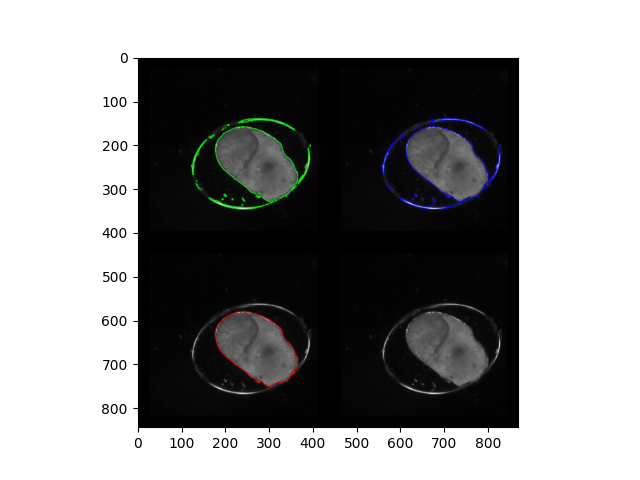
To visualise the results, we now need draw the results on blank canvases and stitch them together.

First we need to generate the canvases:

In [13]: all_ = vuba.bgr(first)

In [14]: l = all_.copy()

In [15]: p = all_.copy()

In [16]: s = all_.copy()

Note that we needed to convert the grayscale frame back to BGR format to enable us to draw coloured shapes. Next we can draw our contours on each of these canvases:

In [17]: vuba.draw_contours(p, parents, -1, (0,0,255), 2)

In [18]: vuba.draw_contours(l, largest, -1, (255,0,0), 2)

In [19]: vuba.draw_contours(s, smallest, -1, (0,255,0), 2)

In [20]: vuba.draw_contours(all_, contours, -1, (0,255,0), 2)

Here we can take advantage of the wrapper draw_contours() which accepts both lists and single numpy arrays. This avoids us having to write for loops for each list of contours. Finally, lets stitch our resultant images together and visualise them:

# Stack the frames so we can view them all at once
In [21]: img1 = np.hstack((all_, p))

In [22]: img2 = np.hstack((l, s))

In [23]: img = np.vstack((img1, img2))

# Resize the final image to a reasonable resolution
In [24]: img = cv2.resize(img, video.resolution)

# And display it
In [25]: plt.imshow(img)
Out[25]: <matplotlib.image.AxesImage at 0x7fd4deeaec50>

Complex filters

In addition to the basic contour filters mentioned above, vuba also supplies several more complex contour filters: Area, Solidity and Eccentricity. Each of these filters permits additional fine-tuning via the use of pre-defined limits, supplied at initiation. This enables us to select specific characteristics for the types of shapes we’d like extracted from a previous set of images.

To demonstrate their usage, we will continue the script started above and add some additional filtering to retrieve small elliptical shapes.

First, let’s create our filters. We will need an area and eccentricity filter:

# Initiate a relatively small area filter
In [26]: area_filter = vuba.Area(min=50, max=300)

# Initiate an eccentricity filter that filters anything out with an eccentricity value greater than 1
In [27]: circle_filter = vuba.Eccentricity(max=1)

Now that we have our filters, we can apply them to the contours we created above:

# Serially combine the filters to extract our shapes
In [28]: small_elliptical = area_filter(circle_filter(contours))

Finally, let’s visualise our results to see what we extracted:

# Draw the shapes on the frame used previously (note the format conversion)
In [29]: elliptical_img = vuba.bgr(first)

In [30]: vuba.draw_contours(elliptical_img, small_elliptical, -1, (0,255,0), 1)

In [31]: plt.imshow(elliptical_img)
Out[31]: <matplotlib.image.AxesImage at 0x7fd4df2d0890>

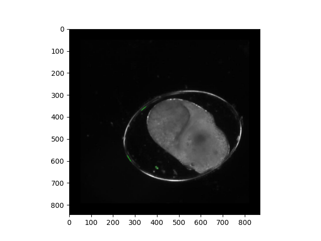
Now, these aren’t much but hopefully show you how you can combine some more complex contour filters to select shapes that satisfy specific criteria.

Contour filters

Basic filters

Complex filters

See also